Lists and Filtering HW

Popcorn Hack 1

import pandas as pd


def find_students_in_range(df, min_score, max_score):
    return df[(df['Score'] >= min_score) & (df['Score'] <= max_score)]

student_data = pd.DataFrame({
    'Name': ['Alice', 'Bob', 'Charlie', 'Diana'],
    'Score': [85, 92, 78, 88]
})

find_students_in_range(student_data, 80, 90)

	Name	Score
0	Alice	85
3	Diana	88

Popcorn Hack 2

def add_letter_grades(df):
    def get_letter(score):
        if score >= 90:
            return 'A'
        elif score >= 80:
            return 'B'
        elif score >= 70:
            return 'C'
        elif score >= 60:
            return 'D'
        else:
            return 'F'
    
    df['Letter'] = df['Score'].apply(get_letter)
    return df


import pandas as pd

student_data = pd.DataFrame({
    'Name': ['Alice', 'Bob', 'Charlie', 'Diana'],
    'Score': [85, 92, 78, 59]
})

add_letter_grades(student_data)

	Name	Score	Letter
0	Alice	85	B
1	Bob	92	A
2	Charlie	78	C
3	Diana	59	F

Popcorn Hack 3

def find_mode(series):
    return series.mode().iloc[0]

import pandas as pd

find_mode(pd.Series([1, 2, 2, 3, 4, 2, 5]))

np.int64(2)

import pandas as pd
import matplotlib.pyplot as plt
import seaborn as sns
import sqlite3
import folium

# Load data
data = pd.read_csv('/home/shawnray/nighthawk/shawnr_2025/datasets/treas_parking_meters_loc_datasd.csv')
data.head()

	zone	area	sub_area	pole	config_id	config_name	date_inventory	lat	lng	sapid
0	Downtown	Core	1000 FIRST AVE	1-1004	49382	Sunday Mode	2021-01-04 00:00:00	32.715904	-117.163929	SS-000031
1	Downtown	Core - Columbia	1000 FIRST AVE	1-1004	9000	2 Hour Max $1.25 HR 8am-6pm Mon-Sat (NFC)	2018-11-11 00:00:00	32.715904	-117.163929	SS-000031
2	Downtown	Core	1000 FIRST AVE	1-1006	49382	Sunday Mode	2021-01-04 00:00:00	32.716037	-117.163930	SS-000031
3	Downtown	Core - Columbia	1000 FIRST AVE	1-1006	9000	2 Hour Max $1.25 HR 8am-6pm Mon-Sat (NFC)	2018-11-11 00:00:00	32.716037	-117.163930	SS-000031
4	Downtown	Core	1000 FIRST AVE	1-1008	49382	Sunday Mode	2021-01-04 00:00:00	32.716169	-117.163931	SS-000031

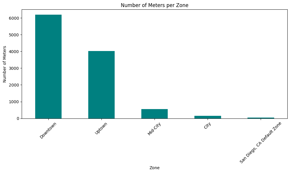
zone_counts = data['zone'].value_counts()

plt.figure(figsize=(10, 6))
zone_counts.plot(kind='bar', color='teal')
plt.title('Number of Meters per Zone')
plt.xlabel('Zone')
plt.ylabel('Number of Meters')
plt.xticks(rotation=45)
plt.tight_layout()
plt.show()

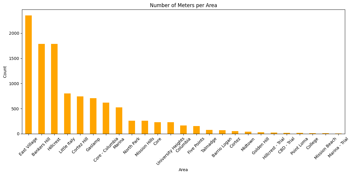
area_counts = data['area'].value_counts().sort_values(ascending=False)
sub_area_counts = data['sub_area'].value_counts().sort_values(ascending=False)

plt.figure(figsize=(12, 6))
area_counts.plot(kind='bar', color='orange')
plt.title('Number of Meters per Area')
plt.xlabel('Area')
plt.ylabel('Count')
plt.xticks(rotation=45)
plt.tight_layout()
plt.show()

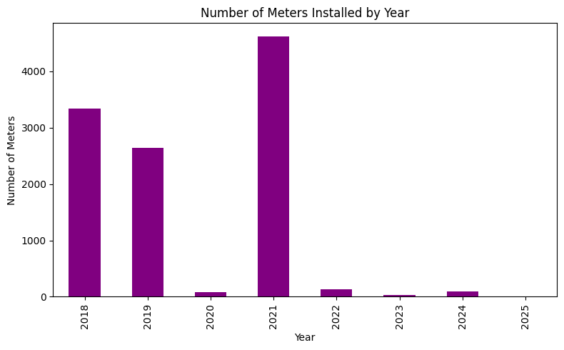
data['date_inventory'] = pd.to_datetime(data['date_inventory'], errors='coerce')
data['inventory_year'] = data['date_inventory'].dt.year

year_counts = data['inventory_year'].value_counts().sort_index()

plt.figure(figsize=(8, 5))
year_counts.plot(kind='bar', color='purple')
plt.title('Number of Meters Installed by Year')
plt.xlabel('Year')
plt.ylabel('Number of Meters')
plt.tight_layout()
plt.show()

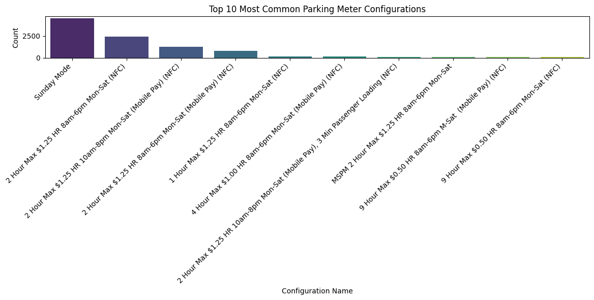
# Top 10 most common configurations
top_configs = data['config_name'].value_counts().head(10)

plt.figure(figsize=(12, 6))
sns.barplot(x=top_configs.index, y=top_configs.values, palette='viridis')

plt.title('Top 10 Most Common Parking Meter Configurations')
plt.xlabel('Configuration Name')
plt.ylabel('Count')
plt.xticks(rotation=45, ha='right')  # Tilt the x-axis labels
plt.tight_layout()
plt.show()

/tmp/ipykernel_1014/91221402.py:5: FutureWarning: 

Passing `palette` without assigning `hue` is deprecated and will be removed in v0.14.0. Assign the `x` variable to `hue` and set `legend=False` for the same effect.

  sns.barplot(x=top_configs.index, y=top_configs.values, palette='viridis')

map_sd = folium.Map(location=[data['lat'].mean(), data['lng'].mean()], zoom_start=13)

for _, row in data.iterrows():
    folium.CircleMarker(
        location=[row['lat'], row['lng']],
        radius=2,
        popup=f"Pole: {row['pole']}<br>Zone: {row['zone']}",
        color='blue',
        fill=True,
        fill_opacity=0.5
    ).add_to(map_sd)

# Show in Jupyter OR save to HTML
map_sd.save('smartpark_map.html')

conn = sqlite3.connect('smartpark_inventory.db')
data.to_sql('meter_inventory', conn, if_exists='replace', index=False)

10964

query1 = """
SELECT zone, COUNT(*) AS meter_count
FROM meter_inventory
GROUP BY zone
ORDER BY meter_count DESC;
"""
pd.read_sql(query1, conn)

	zone	meter_count
0	Downtown	6196
1	Uptown	4017
2	Mid-City	548
3	City	155
4	San Diego, CA Default Zone	48

query2 = """
SELECT config_name, MIN(date_inventory) as first_seen, MAX(date_inventory) as last_seen
FROM meter_inventory
GROUP BY config_name;
"""
pd.read_sql(query2, conn)

	config_name	first_seen	last_seen
0	1 Hour Max $1.25 HR 10am-8pm Mon-Sat (Mobile P...	2018-11-11 00:00:00	2021-03-23 00:00:00
1	1 Hour Max $1.25 HR 8am-4pm Mon-Fri 8am-6pm Sa...	2018-11-11 00:00:00	2018-11-11 00:00:00
2	1 Hour Max $1.25 HR 8am-4pm Mon-Sat (NFC)	2018-11-11 00:00:00	2018-11-11 00:00:00
3	1 Hour Max $1.25 HR 8am-5pm Mon-Sat, No Parkin...	2018-11-11 00:00:00	2018-11-11 00:00:00
4	1 Hour Max $1.25 HR 8am-6pm Mon-Sat (Mobile Pa...	2018-11-11 00:00:00	2020-02-02 00:00:00
...	...	...	...
105	MSPM-PBS 2 Hour Max $1.25 HR 10am-8pm Mon-Sat	2019-12-29 00:00:00	2019-12-29 00:00:00
106	San Diego Default	2018-11-11 00:00:00	2019-12-29 00:00:00
107	Single Space 2 hour meters Petco Special Event...	2019-12-29 00:00:00	2022-09-12 00:00:00
108	Single Space 30 min meters Petco Special Event...	2019-12-29 00:00:00	2019-12-29 00:00:00
109	Sunday Mode	2021-01-04 00:00:00	2021-01-04 00:00:00

110 rows × 3 columns

Comparison: SQL vs Pandas

• Pandas Pros: Easy chaining, good for rapid prototyping, integrates with plotting libraries.
• SQL Pros: Declarative, familiar to database users, better for large structured queries.
• Pandas Cons: Can get messy with complex filters or joins.
• SQL Cons: Harder to visualize data, more verbose syntax for basic operations.

In this project, Pandas was great for quick aggregation and plotting, while SQL was useful for queries like counting meters per zone or filtering by date.